一、Pytorch基本操作考察

使用𝐓𝐞𝐧𝐬𝐨𝐫初始化一个𝟏×𝟑的矩阵𝑴和一个𝟐×𝟏的矩阵𝑵，对两矩阵进行减法操作（要求实现三种不同的形式），给出结果并分析三种方式的不同（如果出现报错，分析报错的原因），同时需要指出在计算过程中发生了什么

1
2
3

import torch
M=torch.Tensor([[1,2,3]])
N=torch.Tensor([[4],[5]])

1 2	#方法一直接相减 print(M-N)

tensor([[-3., -2., -1.],
        [-4., -3., -2.]])

1 2	#方法二使用tensor库中的函数 print(torch.sub(M,N))

tensor([[-3., -2., -1.],
        [-4., -3., -2.]])

1 2	#方法三 print(M.sub(N))

tensor([[-3., -2., -1.],
        [-4., -3., -2.]])

这三种写法分别使用 PyTorch 张量的减法运算符、torch.sub 函数和 Tensor.sub 方法，都会返回新的张量，不会原地修改 M 或 N。M 的形状为 (1, 3)，N 的形状为 (2, 1)；从末尾维度对齐后，每一维的大小相同或其中一个为 1，因此可以广播，结果形状为 (2, 3)。广播不需要先复制出两份完整的 (2, 3) 输入，运算结果则存放在新张量中。这里的 M.sub(N) 没有下划线；如果改为原地操作 M.sub_(N)，就会因为不能把 M 的形状原地扩展为 (2, 3) 而报错。

①利用𝐓𝐞𝐧𝐬𝐨𝐫创建两个大小分别𝟑×𝟐和𝟒×𝟐的随机数矩阵𝑷和𝑸，要求服从均值为0，标准差0.01为的正态分布；②对第二步得到的矩阵𝑸进行形状变换得到𝑸的转置𝑸^T
；③ 对上述得到的矩阵𝑷和矩阵𝑸^T求矩阵相乘

#用𝐓𝐞𝐧𝐬𝐨𝐫创建两个大小分别𝟑×𝟐和𝟒×𝟐的随机数矩阵𝑷和𝑸，服从均值为0，标准差0.01的正态分布
import torch
P=torch.normal(mean=0.0,std=0.01,size=(3,2))
Q=torch.normal(mean=0.0,std=0.01,size=(4,2))
print(P)
print(Q)

tensor([[-0.0082,  0.0247],
        [-0.0128,  0.0130],
        [ 0.0135, -0.0027]])
tensor([[-0.0089,  0.0103],
        [ 0.0092,  0.0080],
        [ 0.0016,  0.0104],
        [ 0.0032, -0.0072]])

1 2	QT=Q.T #得到𝑸的转置 print(QT)

tensor([[-0.0089,  0.0092,  0.0016,  0.0032],
        [ 0.0103,  0.0080,  0.0104, -0.0072]])

1	print(torch.mm(P,QT))

tensor([[ 3.2719e-04,  1.2144e-04,  2.4380e-04, -2.0380e-04],
        [ 2.4757e-04, -1.4374e-05,  1.1514e-04, -1.3395e-04],
        [-1.4752e-04,  1.0277e-04, -7.1371e-06,  6.1853e-05]])

给定公式𝑦3=𝑦1+𝑦2=𝑥^2+𝑥^3，且𝑥=1，利用学习所得到的Tensor的相关知识，求𝑦3对𝑥的梯度，要求在计算过程中，在计算𝑥3时中断梯度的追踪，观察结果并进行原因分析.

import torch
x=torch.tensor(1.0, requires_grad=True)

#y1=x^2 正常计算梯度
y1=x**2
#y2=x^3 但中断梯度追踪
with torch.no_grad():  # 在该上下文管理器中的计算不会追踪梯度
  y2=x**3

y3=y1+y2
y3.backward()
print("梯度dy3/dx:", x.grad)

梯度dy3/dx: tensor(2.)

对于公式 y3 = x^2 + x^3，y1 = x**2 正常记录了反向传播的计算图；y2 = x**3 在 torch.no_grad() 上下文中计算，因此这里的 y2 不记录梯度，y2.requires_grad 为 False。离开该上下文后，y3 = y1 + y2 仍会记录通过 y1 回到 x 的梯度路径；调用 y3.backward() 时，y2 在这次反向传播中被当作常数。于是 x.grad 只得到 x^2 的导数 2x，在 x=1 时为 2.0。如果两项都正常追踪梯度，结果才是 2x + 3x^2 = 5.0。

二、动手实现 logistic 回归

要求动手从0实现 logistic 回归（只借助Tensor和Numpy相关的库）在人工构造的数据集上进行训练和测试，并从loss以及训练集上的准确率等多个角度对结果进行分析（可借助nn.BCELoss或nn.BCEWithLogitsLoss作为损失函数，从零实现二元交叉熵为选作）

首先，生成训练集和测试集

import torch
import numpy as np
import matplotlib.pyplot as plt


# 1. 生成训练、测试数据集

num_inputs = 2  # 创建两类数据点

# 第一类数据点，以 (2, 2) 为中心
x1 = torch.normal(2 * torch.ones(1000, num_inputs), 1)
y1 = torch.ones(1000)

# 第二类数据点，以 (-2, -2) 为中心
x2 = torch.normal(-2 * torch.ones(1000, num_inputs), 1)
y2 = torch.zeros(1000)

# 划分训练集和测试集
# 80% 的数据 (1600个点) 用于训练，20% (400个点) 用于测试
train_index = 800

# 合并成训练集
train_features = torch.cat((x1[:train_index], x2[:train_index]), 0).type(torch.FloatTensor)
train_labels = torch.cat((y1[:train_index], y2[:train_index]), 0).type(torch.FloatTensor)

# 合并成测试集
test_features = torch.cat((x1[train_index:], x2[train_index:]), 0).type(torch.FloatTensor)
test_labels = torch.cat((y1[train_index:], y2[train_index:]), 0).type(torch.FloatTensor)

print(f"训练集大小: {len(train_features)}")
print(f"测试集大小: {len(test_features)}")
print("数据集生成完毕。\n")

训练集大小: 1600
测试集大小: 400
数据集生成完毕。

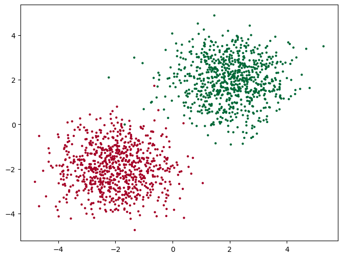
为了方便观察数据分布，这里进行训练集数据的可视化。

# 2. 训练集数据可视化
plt.figure(figsize=(8, 6))
plt.scatter(train_features.data.numpy()[:, 0],
            train_features.data.numpy()[:, 1],
            c=train_labels.data.numpy(),
            s=10, lw=0, cmap='RdYlGn' )
plt.show()

为了方便进行小批量学习，定义数据迭代器

# 第3步：定义数据迭代器
def data_iter(batch_size, features, labels):
    num_examples = len(features)
    indices = list(range(num_examples))
    np.random.shuffle(indices)
    for i in range(0, num_examples, batch_size):
        j = torch.LongTensor(indices[i:min(i + batch_size, num_examples)])
        yield features.index_select(0, j), labels.index_select(0, j)

定义模型、损失函数、优化器

# 第4.1步：定义逻辑回归模型
def logistic_model(X, w, b):
    logits = torch.mm(X, w) + b
    return 1 / (1 + torch.exp(-logits))

# 第4.2步：定义二元交叉熵损失函数
def bce_loss(y_hat, y):
    y = y.view(y_hat.size())
    epsilon = 1e-7 # 防止计算 log(0) 出错
    return -torch.mean(y * torch.log(y_hat + epsilon) + (1 - y) * torch.log(1 - y_hat + epsilon))

# 第4.3步：定义随机梯度下降优化器
def sgd(params, lr):
    for param in params:
        param.data -= lr * param.grad

定义评估函数来计算当前的准确率和平均损失

# 第5步：定义评估函数
def evaluate_performance(features, labels, w, b, loss_fn):
    with torch.no_grad():
        y_hat = logistic_model(features, w, b)
        loss = loss_fn(y_hat, labels.view(y_hat.size()))
        predicted_classes = (y_hat > 0.5).float()
        accuracy = (predicted_classes == labels.view(predicted_classes.size())).float().mean()
    return accuracy.item(), loss.item()

模型参数初始化，给w和b一个随机的初始值

# 第6步：初始化模型参数
w = torch.tensor(np.random.normal(0, 0.01, (num_inputs, 1)), dtype=torch.float32)
b = torch.zeros(1,dtype=torch.float32)

w.requires_grad_(requires_grad=True)
b.requires_grad_(requires_grad=True)

tensor([0.], requires_grad=True)

训练模型

# 第7步：训练模型

lr = 0.01
num_epochs = 20
batch_size = 50

train_losses, test_losses = [], []
train_accuracies, test_accuracies = [], []

for epoch in range(num_epochs):
    # 在每个 epoch 中，遍历所有小批量数据进行学习
    for X, y in data_iter(batch_size, train_features, train_labels):
        y_hat = logistic_model(X, w, b)
        l = bce_loss(y_hat, y)
        l.backward() # 反向传播计算梯度
        sgd([w, b], lr) # 更新参数

        # 清空梯度
        w.grad.data.zero_()
        b.grad.data.zero_()

    # 每个 epoch 结束后，进行评估
    train_acc, train_loss = evaluate_performance(train_features, train_labels, w, b, bce_loss)
    test_acc, test_loss = evaluate_performance(test_features, test_labels, w, b, bce_loss)

    train_losses.append(train_loss)
    test_losses.append(test_loss)
    train_accuracies.append(train_acc)
    test_accuracies.append(test_acc)

    print(f'Epoch {epoch + 1}, Train Loss: {train_loss:.4f}, Train Acc: {train_acc:.3f}, Test Loss: {test_loss:.4f}, Test Acc: {test_acc:.3f}')

print("训练完成！\n")

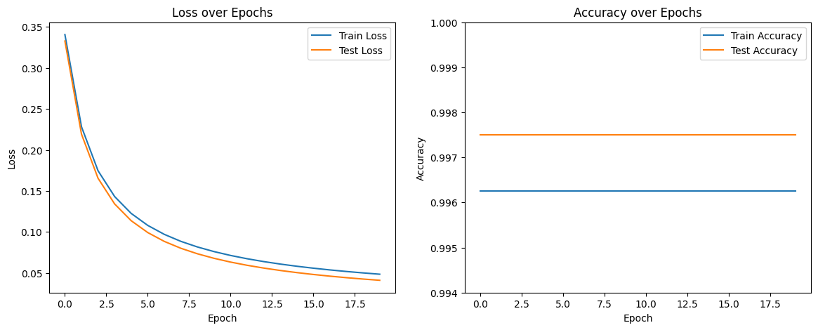
Epoch 1, Train Loss: 0.3407, Train Acc: 0.996, Test Loss: 0.3328, Test Acc: 0.998
Epoch 2, Train Loss: 0.2283, Train Acc: 0.996, Test Loss: 0.2193, Test Acc: 0.998
Epoch 3, Train Loss: 0.1746, Train Acc: 0.996, Test Loss: 0.1654, Test Acc: 0.998
Epoch 4, Train Loss: 0.1432, Train Acc: 0.996, Test Loss: 0.1341, Test Acc: 0.998
Epoch 5, Train Loss: 0.1226, Train Acc: 0.996, Test Loss: 0.1137, Test Acc: 0.998
Epoch 6, Train Loss: 0.1079, Train Acc: 0.996, Test Loss: 0.0992, Test Acc: 0.998
Epoch 7, Train Loss: 0.0970, Train Acc: 0.996, Test Loss: 0.0884, Test Acc: 0.998
Epoch 8, Train Loss: 0.0885, Train Acc: 0.996, Test Loss: 0.0800, Test Acc: 0.998
Epoch 9, Train Loss: 0.0816, Train Acc: 0.996, Test Loss: 0.0733, Test Acc: 0.998
Epoch 10, Train Loss: 0.0760, Train Acc: 0.996, Test Loss: 0.0678, Test Acc: 0.998
Epoch 11, Train Loss: 0.0713, Train Acc: 0.996, Test Loss: 0.0632, Test Acc: 0.998
Epoch 12, Train Loss: 0.0673, Train Acc: 0.996, Test Loss: 0.0593, Test Acc: 0.998
Epoch 13, Train Loss: 0.0638, Train Acc: 0.996, Test Loss: 0.0559, Test Acc: 0.998
Epoch 14, Train Loss: 0.0608, Train Acc: 0.996, Test Loss: 0.0529, Test Acc: 0.998
Epoch 15, Train Loss: 0.0581, Train Acc: 0.996, Test Loss: 0.0504, Test Acc: 0.998
Epoch 16, Train Loss: 0.0557, Train Acc: 0.996, Test Loss: 0.0481, Test Acc: 0.998
Epoch 17, Train Loss: 0.0536, Train Acc: 0.996, Test Loss: 0.0460, Test Acc: 0.998
Epoch 18, Train Loss: 0.0517, Train Acc: 0.996, Test Loss: 0.0442, Test Acc: 0.998
Epoch 19, Train Loss: 0.0500, Train Acc: 0.996, Test Loss: 0.0425, Test Acc: 0.998
Epoch 20, Train Loss: 0.0484, Train Acc: 0.996, Test Loss: 0.0410, Test Acc: 0.998
训练完成！

训练结束，画图分析学习成果

# 第8步：结果可视化与分析
plt.figure(figsize=(14, 5))

# 绘制损失曲线
plt.subplot(1, 2, 1)
plt.plot(train_losses, label='Train Loss')
plt.plot(test_losses, label='Test Loss')
plt.title('Loss over Epochs')
plt.xlabel('Epoch')
plt.ylabel('Loss')
plt.legend()

# 绘制准确率曲线
plt.subplot(1, 2, 2)
plt.plot(train_accuracies, label='Train Accuracy')
plt.plot(test_accuracies, label='Test Accuracy')
plt.title('Accuracy over Epochs')
plt.xlabel('Epoch')
plt.ylabel('Accuracy')
plt.ylim(0.994, 1.0)
plt.legend()

plt.show()

--- 正在绘制结果图表... ---

逻辑回归训练结果：训练集与测试集损失随轮次下降，准确率曲线保持水平，测试集略高于训练集。

通过从零开始手动实现逻辑回归，结果显示，模型的损失（Loss）在最初几轮训练中就迅速下降并趋于稳定，同时训练集准确率（Accuracy）也快速达到了接近100%的水平。这成功地验证了手动实现的sigmoid函数、二元交叉熵损失以及梯度下降优化器是正确且有效的。

利用torch.nn 实现 logistic 回归在人工构造的数据集上进行训练和测试，并对结果进行分析，并从loss以及训练集上的准确率等多个角度对结果进行分析

准备数据

import torch
import numpy as np
import matplotlib.pyplot as plt
import torch.utils.data as Data
from torch.nn import init
from torch import nn

#1. 使用 DataLoader 读取数据
batch_size = 50
train_dataset = Data.TensorDataset(train_features, train_labels)
train_loader = Data.DataLoader(dataset=train_dataset, batch_size=batch_size, shuffle=True)

test_dataset = Data.TensorDataset(test_features, test_labels)
test_loader = Data.DataLoader(dataset=test_dataset, batch_size=batch_size, shuffle=False)

nn.Module搭建模型

#2. 使用 nn.Module 定义模型
from torch import nn

class LogisticRegressionNN(nn.Module):
    def __init__(self, n_features):
        super(LogisticRegressionNN, self).__init__()
        self.linear = nn.Linear(n_features, 1)
        self.sigmoid = nn.Sigmoid()
    def forward(self, x):
        x = self.linear(x)
        x = self.sigmoid(x)
        return x

初始化模型，定义损失函数，优化器

# 3.初始化模型，定义损失函数、优化器

model = LogisticRegressionNN(num_inputs)

criterion = nn.BCELoss()

optimizer = torch.optim.SGD(model.parameters(), lr=0.001)

定义评估函数

# 4.定义评估函数
def evaluate_nn(loader, model, criterion):
    model.eval()
    total_loss = 0
    correct = 0
    total = 0
    with torch.no_grad():
        for features, labels in loader:
            outputs = model(features)
            loss = criterion(outputs, labels.view(-1, 1))
            total_loss += loss.item() * len(labels)

            predicted = (outputs > 0.5).float()
            total += len(labels)
            correct += (predicted == labels.view(-1, 1)).sum().item()

    model.train()
    return correct / total, total_loss / total

训练模型

# 5.训练模型
num_epochs = 20
train_losses_nn, test_losses_nn = [], []
train_accuracies_nn, test_accuracies_nn = [], []

for epoch in range(num_epochs):
    model.train()
    for features, labels in train_loader:
        outputs = model(features)
        loss = criterion(outputs, labels.view(-1, 1))

        optimizer.zero_grad() #清除旧梯度
        loss.backward() #计算新梯度
        optimizer.step() #更新参数

    # 每个 epoch 结束后，评估模型
    train_acc, train_loss = evaluate_nn(train_loader, model, criterion)
    test_acc, test_loss = evaluate_nn(test_loader, model, criterion)

    train_losses_nn.append(train_loss)
    test_losses_nn.append(test_loss)
    train_accuracies_nn.append(train_acc)
    test_accuracies_nn.append(test_acc)

    print(f'Epoch {epoch + 1}, Train Loss: {train_loss:.4f}, Train Acc: {train_acc:.3f}, Test Loss: {test_loss:.4f}, Test Acc: {test_acc:.3f}')

print("nn 模型训练完成！\n")

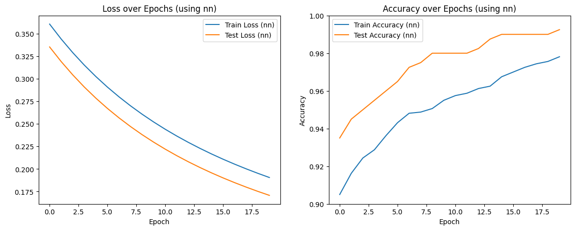
Epoch 1, Train Loss: 0.3608, Train Acc: 0.905, Test Loss: 0.3354, Test Acc: 0.935
Epoch 2, Train Loss: 0.3442, Train Acc: 0.916, Test Loss: 0.3192, Test Acc: 0.945
Epoch 3, Train Loss: 0.3291, Train Acc: 0.924, Test Loss: 0.3045, Test Acc: 0.950
Epoch 4, Train Loss: 0.3153, Train Acc: 0.929, Test Loss: 0.2910, Test Acc: 0.955
Epoch 5, Train Loss: 0.3026, Train Acc: 0.936, Test Loss: 0.2786, Test Acc: 0.960
Epoch 6, Train Loss: 0.2909, Train Acc: 0.943, Test Loss: 0.2672, Test Acc: 0.965
Epoch 7, Train Loss: 0.2801, Train Acc: 0.948, Test Loss: 0.2568, Test Acc: 0.973
Epoch 8, Train Loss: 0.2701, Train Acc: 0.949, Test Loss: 0.2471, Test Acc: 0.975
Epoch 9, Train Loss: 0.2608, Train Acc: 0.951, Test Loss: 0.2381, Test Acc: 0.980
Epoch 10, Train Loss: 0.2522, Train Acc: 0.955, Test Loss: 0.2298, Test Acc: 0.980
Epoch 11, Train Loss: 0.2441, Train Acc: 0.958, Test Loss: 0.2220, Test Acc: 0.980
Epoch 12, Train Loss: 0.2366, Train Acc: 0.959, Test Loss: 0.2148, Test Acc: 0.980
Epoch 13, Train Loss: 0.2295, Train Acc: 0.961, Test Loss: 0.2080, Test Acc: 0.983
Epoch 14, Train Loss: 0.2229, Train Acc: 0.963, Test Loss: 0.2017, Test Acc: 0.988
Epoch 15, Train Loss: 0.2167, Train Acc: 0.968, Test Loss: 0.1957, Test Acc: 0.990
Epoch 16, Train Loss: 0.2109, Train Acc: 0.970, Test Loss: 0.1901, Test Acc: 0.990
Epoch 17, Train Loss: 0.2054, Train Acc: 0.973, Test Loss: 0.1849, Test Acc: 0.990
Epoch 18, Train Loss: 0.2002, Train Acc: 0.974, Test Loss: 0.1799, Test Acc: 0.990
Epoch 19, Train Loss: 0.1953, Train Acc: 0.976, Test Loss: 0.1752, Test Acc: 0.990
Epoch 20, Train Loss: 0.1906, Train Acc: 0.978, Test Loss: 0.1708, Test Acc: 0.993
nn 模型训练完成！

训练结束，画图分析学习成果

# 6.结果可视化与分析
plt.figure(figsize=(14, 5))
plt.subplot(1, 2, 1)
plt.plot(train_losses_nn, label='Train Loss (nn)')
plt.plot(test_losses_nn, label='Test Loss (nn)')
plt.title('Loss over Epochs (using nn)')
plt.xlabel('Epoch')
plt.ylabel('Loss')
plt.legend()
plt.subplot(1, 2, 2)
plt.plot(train_accuracies_nn, label='Train Accuracy (nn)')
plt.plot(test_accuracies_nn, label='Test Accuracy (nn)')
plt.title('Accuracy over Epochs (using nn)')
plt.xlabel('Epoch')
plt.ylabel('Accuracy')
plt.ylim(0.9, 1.0)
plt.legend()
plt.show()

torch.nn逻辑回归训练曲线：训练与测试损失持续下降，准确率分别升至约97.8%和99.3%。

使用torch.nn模块实现逻辑回归同样在人工数据集上获得了极高的准确率和极低的损失，其结果与从零实现版本高度一致。通过使用标准化模块高效地达到了同样的目标。

三、动手实现 softmax回归

要求动手从0实现 softmax回归（只借助Tensor和Numpy相关的库）在Fashion-MNIST数据
集上进行训练和测试，并从loss、训练集以及测试集上的准确率等多个角度对结果进行分析
（要求从零实现交叉熵损失函数）

加载 Fashion-MNIST 数据集

import torch
import torchvision
import torchvision.transforms as transforms
import numpy as np
import matplotlib.pyplot as plt
import time

# 第1步：加载 Fashion-MNIST 数据集

batch_size = 256


transform = transforms.ToTensor()

# 下载并加载训练集
mnist_train = torchvision.datasets.FashionMNIST(
    root="./data",
    train=True,             # 加载训练集
    download=True,
    transform=transform
)

# 下载并加载测试集
mnist_test = torchvision.datasets.FashionMNIST(
    root="./data",
    train=False,            # 加载测试集
    download=True,
    transform=transform
)


train_iter = torch.utils.data.DataLoader(mnist_train, batch_size=batch_size, shuffle=True)
test_iter = torch.utils.data.DataLoader(mnist_test, batch_size=batch_size, shuffle=False)

print("数据集加载完成！\n")

数据集加载完成！

拿出几张照片及其对应的标签进行可视化，直观感受模型要处理的输入及需要达到的目标

# --- 第2步：可视化部分数据集 ---
def get_fashion_mnist_labels(labels):
    #将数字标签转换为文本标签
    text_labels = ['t-shirt', 'trouser', 'pullover', 'dress', 'coat',
                   'sandal', 'shirt', 'sneaker', 'bag', 'ankle boot']
    return [text_labels[int(i)] for i in labels]

def show_fashion_mnist(images, labels):
    #显示图像和对应的标签
    _, figs = plt.subplots(1, len(images), figsize=(12, 12))
    for f, img, lbl in zip(figs, images, labels):
        f.imshow(img.view((28, 28)).numpy(), cmap='gray')
        f.set_title(lbl)
        f.axes.get_xaxis().set_visible(False)
        f.axes.get_yaxis().set_visible(False)
    plt.show()


X, y = next(iter(train_iter))

show_fashion_mnist(X[0:10], get_fashion_mnist_labels(y[0:10]))

10张服饰灰度样例，从左到右标注为：包、凉鞋、套头衫、凉鞋、凉鞋、连衣裙、衬衫、连衣裙、衬衫、套头衫。

定义模型，损失函数，优化器，初始化模型参数

# 第3.1步：初始化模型参数

num_inputs = 784  # 28 * 28
num_outputs = 10 # 10分类问题

W = torch.tensor(np.random.normal(0, 0.01, (num_inputs, num_outputs)), dtype=torch.float32)
b = torch.zeros(num_outputs, dtype=torch.float32)

W.requires_grad_(requires_grad=True)
b.requires_grad_(requires_grad=True)

# 第3.2步：实现 Softmax 运算
def softmax(X):
    X_exp = torch.exp(X)
    partition = X_exp.sum(dim=1, keepdim=True)
    return X_exp / partition

# 第3.3步：定义模型
def net(X):

    linear_output = torch.mm(X.view((-1, num_inputs)), W) + b
    return softmax(linear_output)

# 第3.4步：定义损失函数 (交叉熵)
def cross_entropy(y_hat, y):
    # y_hat 是模型的输出(batch_size, 10)，y 是真实标签(batch_size)
    # y_hat.gather(1, y.view(-1, 1)) 会挑出每个样本对应正确标签的那个概率值
    return -torch.log(y_hat.gather(1, y.view(-1, 1)))

# 第3.5步：定义优化器
def sgd(params, lr, batch_size):
    for param in params:
        param.data -= lr * param.grad / batch_size

定义评估函数

# 第4步：定义精度评估函数
def evaluate_accuracy(data_iter, net_fn):
    acc_sum, n = 0.0, 0
    with torch.no_grad():
        for X, y in data_iter:
            # net_fn(X).argmax(dim=1) 找出预测的类别
            acc_sum += (net_fn(X).argmax(dim=1) == y).float().sum().item()
            n += y.shape[0]
    return acc_sum / n

训练模型

# 第5步：训练模型

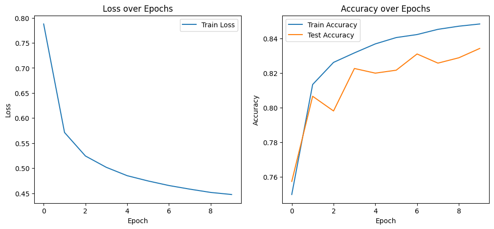
num_epochs = 10
lr = 0.1

train_losses, test_losses = [], []
train_accuracies, test_accuracies = [], []

def train_epoch(net, train_iter, loss, updater):

    train_l_sum, train_acc_sum, n = 0.0, 0.0, 0
    for X, y in train_iter:
        y_hat = net(X)
        l = loss(y_hat, y)
        l.sum().backward()
        updater([W, b], lr, batch_size)

        W.grad.data.zero_()
        b.grad.data.zero_()

        train_l_sum += l.sum().item()
        train_acc_sum += (y_hat.argmax(dim=1) == y).sum().item()
        n += y.shape[0]
    return train_acc_sum / n, train_l_sum / n

for epoch in range(num_epochs):
    # 训练
    train_acc, train_loss = train_epoch(net, train_iter, cross_entropy, sgd)

    # 在测试集上评估
    test_acc = evaluate_accuracy(test_iter, net)

    train_accuracies.append(train_acc)
    train_losses.append(train_loss)
    test_accuracies.append(test_acc)

    print(f'Epoch {epoch + 1}, Train Loss: {train_loss:.4f}, Train Acc: {train_acc:.3f}, Test Acc: {test_acc:.3f}')

print("训练完成！\n")

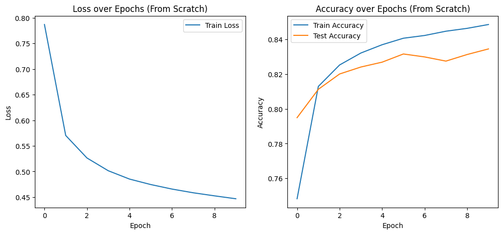
Epoch 1, Train Loss: 0.7870, Train Acc: 0.748, Test Acc: 0.795
Epoch 2, Train Loss: 0.5703, Train Acc: 0.813, Test Acc: 0.811
Epoch 3, Train Loss: 0.5263, Train Acc: 0.825, Test Acc: 0.820
Epoch 4, Train Loss: 0.5015, Train Acc: 0.832, Test Acc: 0.824
Epoch 5, Train Loss: 0.4852, Train Acc: 0.837, Test Acc: 0.827
Epoch 6, Train Loss: 0.4745, Train Acc: 0.841, Test Acc: 0.832
Epoch 7, Train Loss: 0.4656, Train Acc: 0.842, Test Acc: 0.830
Epoch 8, Train Loss: 0.4584, Train Acc: 0.845, Test Acc: 0.827
Epoch 9, Train Loss: 0.4524, Train Acc: 0.846, Test Acc: 0.831
Epoch 10, Train Loss: 0.4467, Train Acc: 0.848, Test Acc: 0.834
训练完成！

结果可视化分析学习结果

# 第6步：结果可视化与分析

plt.figure(figsize=(12, 5))

# 绘制损失曲线
plt.subplot(1, 2, 1)
plt.plot(train_losses, label='Train Loss')
plt.title('Loss over Epochs (From Scratch)')
plt.xlabel('Epoch')
plt.ylabel('Loss')
plt.legend()

# 绘制准确率曲线
plt.subplot(1, 2, 2)
plt.plot(train_accuracies, label='Train Accuracy')
plt.plot(test_accuracies, label='Test Accuracy')
plt.title('Accuracy over Epochs (From Scratch)')
plt.xlabel('Epoch')
plt.ylabel('Accuracy')
plt.legend()

plt.show()

从零实现Softmax回归：训练损失持续下降，训练准确率升至约85%，测试准确率中途略有回落，最终约83.5%。

在Fashion-MNIST多分类任务上，从零实现的Softmax回归模型表现出了良好的学习能力。从结果损失曲线和准确率曲线图可以看出，模型的训练损失持续稳定下降，而训练集和测试集的准确率都在稳步攀升，这表明手动实现的softmax函数、多类交叉熵损失和优化算法能够有效工作。

利用torch.nn实现 softmax 回归在Fashion-MNIST数据集上进行训练和测试，并从loss，训练集以及测试集上的准确率等多个角度对结果进行分析

首先准备数据

import torch
import torchvision
import torchvision.transforms as transforms
import numpy as np
import matplotlib.pyplot as plt
import time

# 第1步：加载 Fashion-MNIST 数据集

batch_size = 256


transform = transforms.ToTensor()

# 下载并加载训练集
mnist_train = torchvision.datasets.FashionMNIST(
    root="./data",
    train=True,             # 加载训练集
    download=True,
    transform=transform
)

# 下载并加载测试集
mnist_test = torchvision.datasets.FashionMNIST(
    root="./data",
    train=False,            # 加载测试集
    download=True,
    transform=transform
)


train_iter = torch.utils.data.DataLoader(mnist_train, batch_size=batch_size, shuffle=True)
test_iter = torch.utils.data.DataLoader(mnist_test, batch_size=batch_size, shuffle=False)

print("数据集加载完成！\n")

数据集加载完成！

使用torch.nn搭建模型

# 第1步 & 2步：定义并初始化模型
from torch import nn


net_nn = nn.Sequential(
    nn.Flatten(),
    nn.Linear(784, 10)
)

def init_weights(m):
    if type(m) == nn.Linear:
        nn.init.normal_(m.weight, std=0.01)

net_nn.apply(init_weights)

Sequential(
  (0): Flatten(start_dim=1, end_dim=-1)
  (1): Linear(in_features=784, out_features=10, bias=True)
)

定义损失函数和优化器

1
2
3

# 第3步：定义损失函数和优化器
loss = nn.CrossEntropyLoss() #在内部自动完成 softmax 计算和交叉熵损失计算。
optimizer = torch.optim.SGD(net_nn.parameters(), lr=0.1)

标准化的训练流程

# 第4步：训练模型

def train_epoch_nn(net, train_iter, loss_fn, optim):
    net.train() # 切换到训练模式
    train_l_sum, train_acc_sum, n = 0.0, 0.0, 0
    for X, y in train_iter:
        y_hat = net(X)
        l = loss_fn(y_hat, y)
        optim.zero_grad()
        l.backward()
        optim.step()

        train_l_sum += l.item() * len(y)
        train_acc_sum += (y_hat.argmax(dim=1) == y).sum().item()
        n += y.shape[0]
    return train_acc_sum / n, train_l_sum / n

def evaluate_accuracy_nn(net, data_iter):# 这里的评估函数与第一部分手动实现的评估函数相同，可以直接使用第一部分的评估函数，为了代码更加清晰这里选择重写一遍。
    net.eval() # 切换到评估模式
    acc_sum, n = 0.0, 0
    with torch.no_grad():
        for X, y in data_iter:
            acc_sum += (net(X).argmax(dim=1) == y).float().sum().item()
            n += y.shape[0]
    return acc_sum / n

train_losses_nn, train_accuracies_nn = [], []
test_accuracies_nn = []

for epoch in range(num_epochs):
    train_acc, train_loss = train_epoch_nn(net_nn, train_iter, loss, optimizer)
    test_acc = evaluate_accuracy_nn(net_nn, test_iter)

    train_accuracies_nn.append(train_acc)
    train_losses_nn.append(train_loss)
    test_accuracies_nn.append(test_acc)

    print(f'Epoch {epoch + 1}, Train Loss: {train_loss:.4f}, Train Acc: {train_acc:.3f}, Test Acc: {test_acc:.3f}')

print("训练完成！\n")

Epoch 1, Train Loss: 0.7877, Train Acc: 0.750, Test Acc: 0.757
Epoch 2, Train Loss: 0.5712, Train Acc: 0.813, Test Acc: 0.807
Epoch 3, Train Loss: 0.5243, Train Acc: 0.826, Test Acc: 0.798
Epoch 4, Train Loss: 0.5017, Train Acc: 0.832, Test Acc: 0.823
Epoch 5, Train Loss: 0.4850, Train Acc: 0.837, Test Acc: 0.820
Epoch 6, Train Loss: 0.4745, Train Acc: 0.841, Test Acc: 0.822
Epoch 7, Train Loss: 0.4654, Train Acc: 0.842, Test Acc: 0.831
Epoch 8, Train Loss: 0.4582, Train Acc: 0.845, Test Acc: 0.826
Epoch 9, Train Loss: 0.4516, Train Acc: 0.847, Test Acc: 0.829
Epoch 10, Train Loss: 0.4475, Train Acc: 0.848, Test Acc: 0.834
训练完成！

结果可视化分析学习结果

# 第5步：结果可视化与分析

plt.figure(figsize=(12, 5))

# 绘制损失曲线
plt.subplot(1, 2, 1)
plt.plot(train_losses_nn, label='Train Loss')
plt.title('Loss over Epochs')
plt.xlabel('Epoch')
plt.ylabel('Loss')
plt.legend()

# 绘制准确率曲线
plt.subplot(1, 2, 2)
plt.plot(train_accuracies_nn, label='Train Accuracy')
plt.plot(test_accuracies_nn, label='Test Accuracy')
plt.title('Accuracy over Epochs')
plt.xlabel('Epoch')
plt.ylabel('Accuracy')
plt.legend()

plt.show()

torch.nn实现Softmax回归：训练损失持续下降，训练准确率升至约85%，测试准确率波动上升至约83.4%。

通过torch.nn实现Softmax回归在Fashion-MNIST数据集上轻松复现并验证了从零实现的版本的效果。nn.CrossEntropyLoss则巧妙地将softmax计算和损失函数合二为一，使代码更简洁且数值上更稳定，最终结果显示，损失随着训练轮数下降，模型同样达到了理想的准确率。

校订记录（2026-10-09）：本页从原文迁入后，依据 PyTorch 官方文档校正了广播与 torch.no_grad() 的说明；原始代码、实验输出和原文日期保留，未重新运行训练实验。参考：广播规则、no_grad。

PyTorch基本操作实验

一、Pytorch基本操作考察

二、动手实现 logistic 回归

三、动手实现 softmax回归

评论

去哪里？

搜索

图像来源

节拍

后台操作小抄